Chapter 1: Get Started
Submission Requirement
You are required to submit a report for this lab. Please follow the instructions below, complete “Lab1 report” and submit it on Canvas.
1.1. Software Installation
1.1.1 R and RStudio
R is the based app to process R programming language, and RStudio
integrates with R to provide further functionality such as graphical
user interface (GUI). We need to install both R and
RStudio for this workshop.
Note: there are R and RStudio installed in the
computer lab. Please use the PCs in the lab if you cannot install.
1.1.2 Install R
We will install R first.
Windows users:
- Please go to the website: https://cran.rstudio.com/
- Download and install R
- Click Download R for Windows
- Click install R for the first time
- Download R-4.5.1 for Windows (Remember the folder where you saved it!!)
- Go to the folder where you save the file “R-4.5.1-win.exe”, double click to run the installation, use default settings, click Next until the end
- Finish
Mac users:
- Please go to the website: https://cran.rstudio.com/
- Click Download R for macOS
- Under the Latest release, download the version that is suitable for your machine (“R-4.5.1-arm64.pkg” or “R-4.5.1-x86_64.pkg”) –> save
- Go to the folder where you save the file, run the installation, use default settings, click Next until the end
- Finish
1.1.3 Install RStudio
Next, we will install RStudio, the GUI of R.
Windows users:
- Please go to: https://posit.co/download/rstudio-desktop/
- Under 2: Install RStudio click on Download RStudio desktop for windows, then Save
- Go to the folder where you download the file “RStudio-xxxx.exe”
- Run the installation, use default settings, click
Next until the end
- Finish
Mac users:
- Please go to: https://posit.co/download/rstudio-desktop/
- Scroll down
- look for macOS 13+, click RStudio-2025.05.1-513.dmg and save
- Go to the folder where you download the file
- Run the installation, use default settings, click Next until the end
- Finish
1.2. Good Practice - Organizing Folders
It happens to me all the time that my course A files are mixed with course B’s. To make things easier, I highly recommend organizing your folders in the following way:
- Create a folder specifically for this course (e.g., Geoviz).
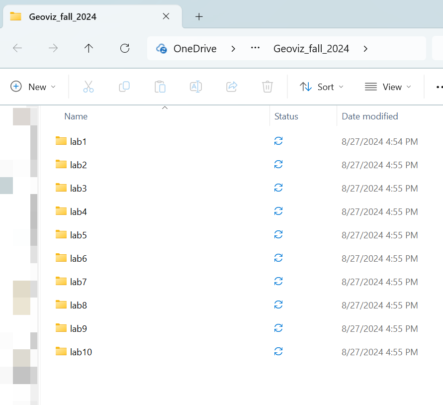
- Under the course folder, create a series of sub-folders for different labs and assignments separately, for example, folders with “lab1”, “lab2”, “lab3”…..”assignment1”, “assignment2”….(see Figure 1.1)
- For different tasks, work in their specific folders. For example,
for this lab, you should work in the “lab1” folder under the
“Geoviz_fall_2024” course folder.
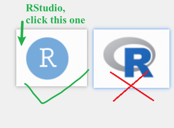
1.3. Launching RStudio
Earlier, we have installed both R and RStudio. But for this and all future labs, we only need to run RStudio. This is because R is the hidden computing infrastructure while RStudio is the interface.
Run RStudio.
If it is the first time to run RStudio, it may ask you to select the version of R to use. Use the default option “64-bit version of R”, click “OK”. “Enable automated crash reporting” –> “Yes”
After launching RStudio, you will see the following interface (Figure
1.3). 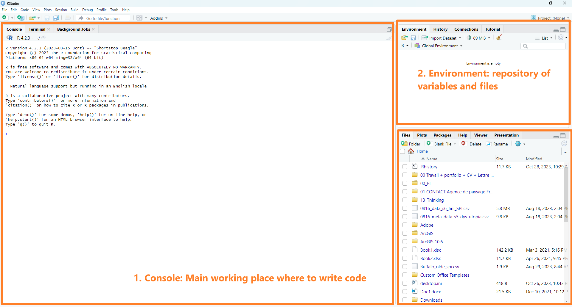
1.3.1 Create a project
Before creating a project, please make sure that you have already
created your course folder and the sub-folder “lab1” as
mentioned in Section 2: Good practice.
In RStudio menu –> File –> New Project –> Existing
Directory –> Browse & Navigate to the course folder, then the
sub-folder “lab1” –> Double clicks to go inside of
the folder “lab1” –> Open –> Create Project
Note: we will need to repeat this to create projects for future
labs and assignments.
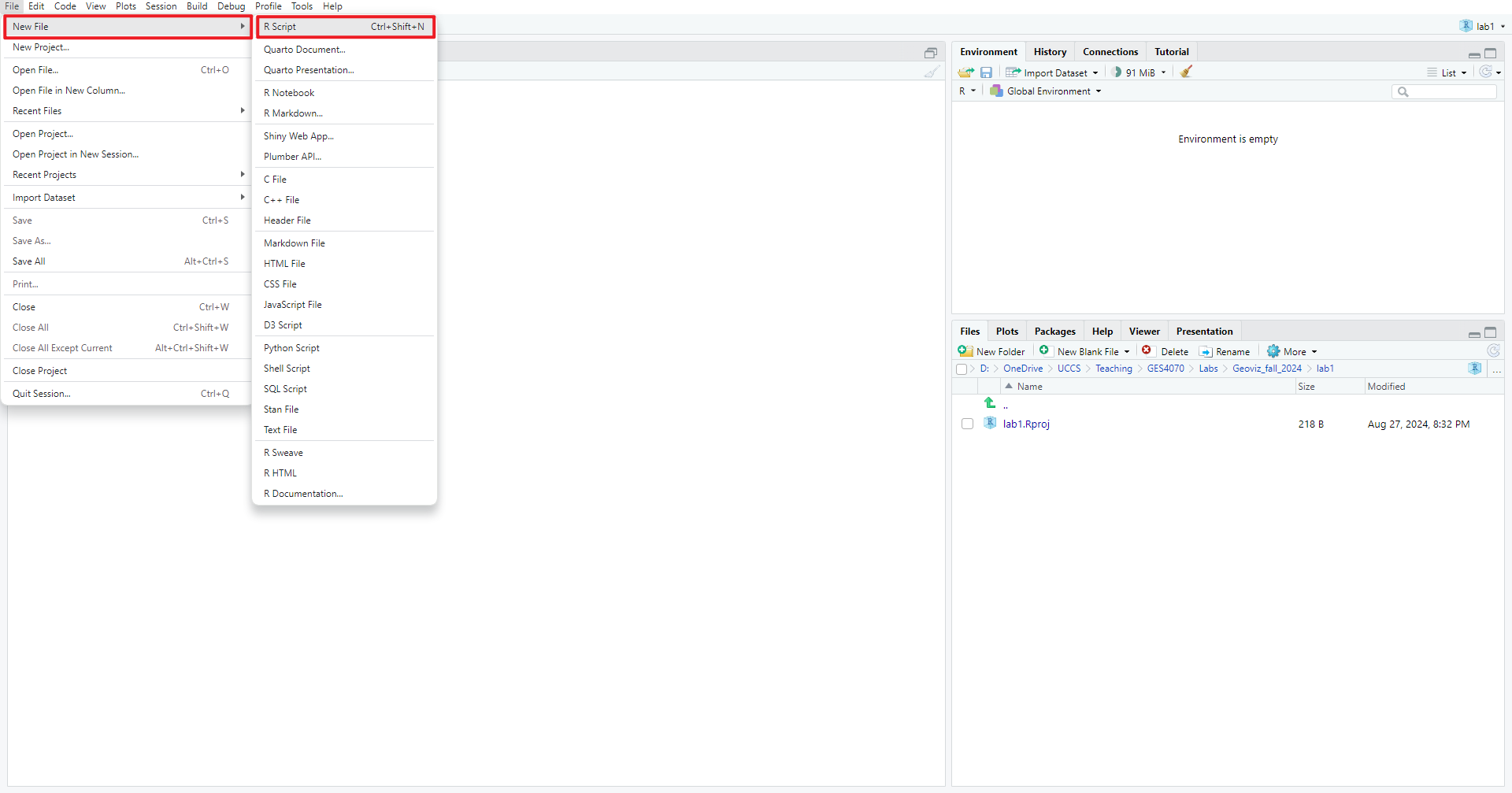
1.3.1 Create a new script
A script is a sequence of instructions that can be executed by a computer or programming language (in our case, R). To create a new script, in RStudio menu –> New File –> R Script (see Figure 1.4)
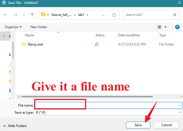
Then, we also need to save the script to the “lab1” folder. File
–> Save –> Specify File Name –> Save (see Figure 1.5)
After creating and saving the new script, you should see something
similar to Figure 1.6.
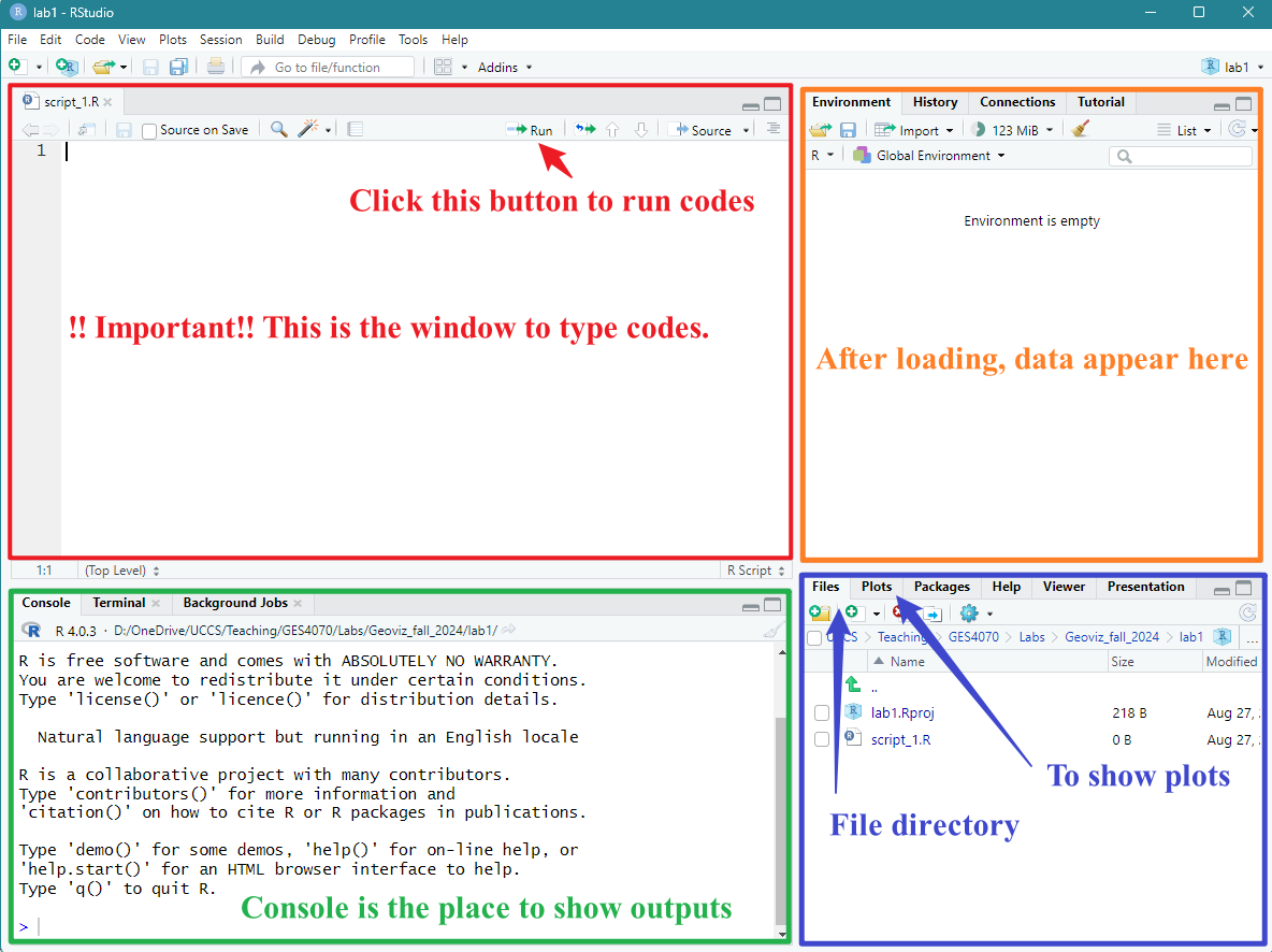
Let’s try to coding now. First, let’s ask the machine to do math for us.
- Type the following command in the top-left window (red in Figure 1.6)
- Select that line
- click run
2+5+8## [1] 15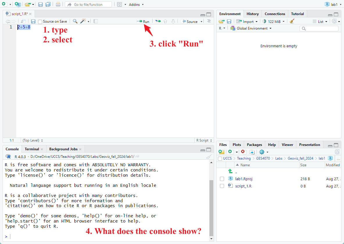 Next, let’s asking the machine
to print some words for us. Type the following command and run it.
Hint: to run codes, please select the lines you want to run and
click “Run”
Next, let’s asking the machine
to print some words for us. Type the following command and run it.
Hint: to run codes, please select the lines you want to run and
click “Run”
print("GES Geovisualization")## [1] "GES Geovisualization"Good Coding Practice:
- Always start a new line when writing a new command;
- In R & RStudio, scripts are !!case-sensitive!! Changing the capitalization of codes can run into errors.
- When creating new variables, avoid spaces by using underscore “\(_\)”. For example, “city\(_\)boundary” is a good variable name, but “city boundary” will cause errors.
1.4. Let’s start mapping!
tmap is a commonly used package in R for mapping. We install this package first. Type the command in your script and click “run”.
install.packages("tmap")Then, we load the tmap package. Again, type –> select –> run
# load "tmap"
library(tmap)
1.4.1. Hello World!
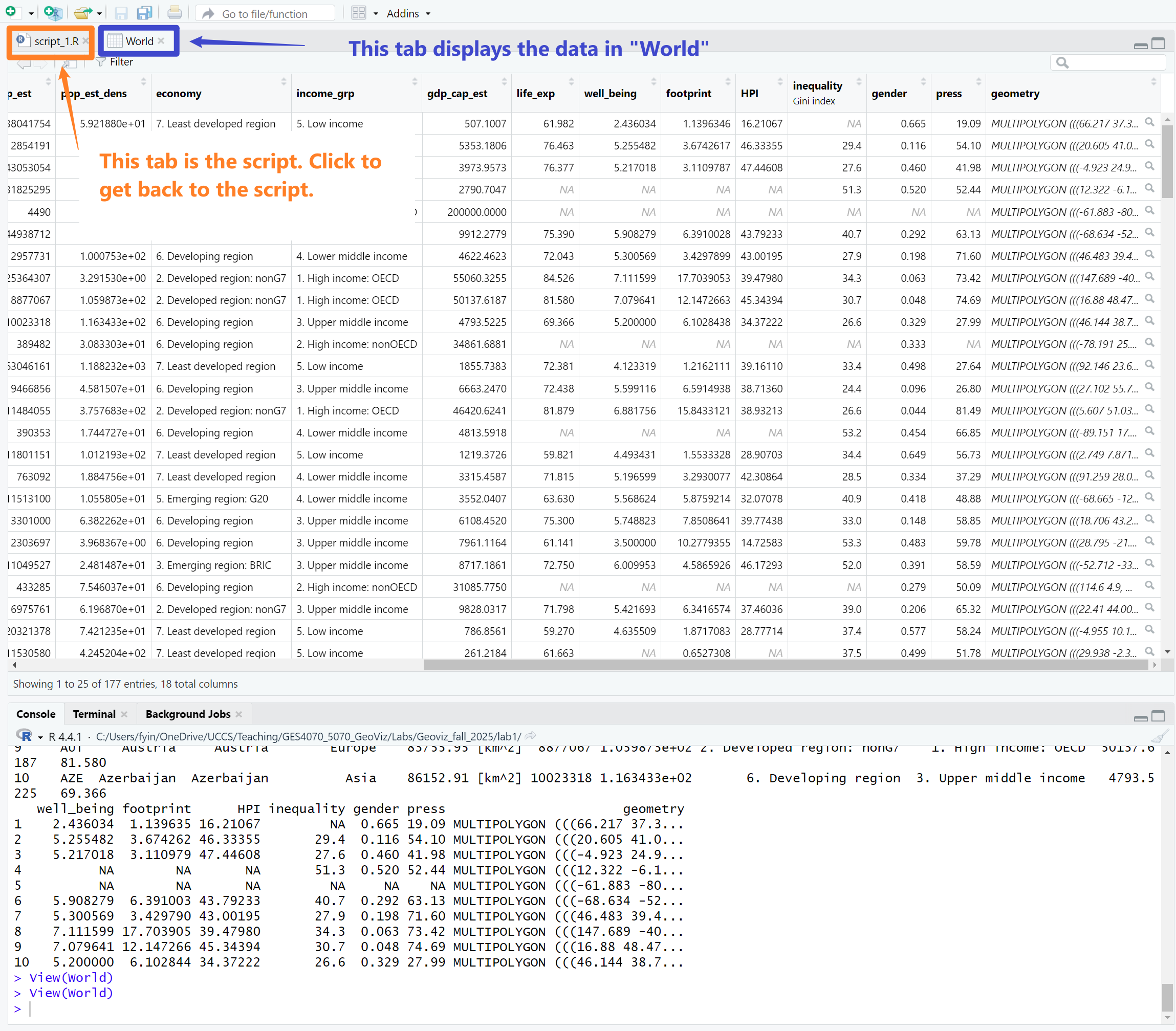
The package tmap itself has a dataset on the world’s countries. Let’s load the data first. On the top-right panel ‘Global Environment’, there is a variable called ‘World’. You can see the detailed data in the variable by clicking on it.
# load the world data
data("World")
## Warning in data("World"): data set 'World' not found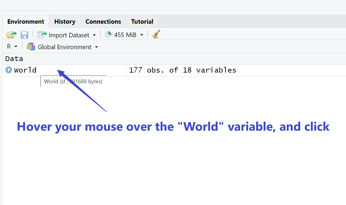
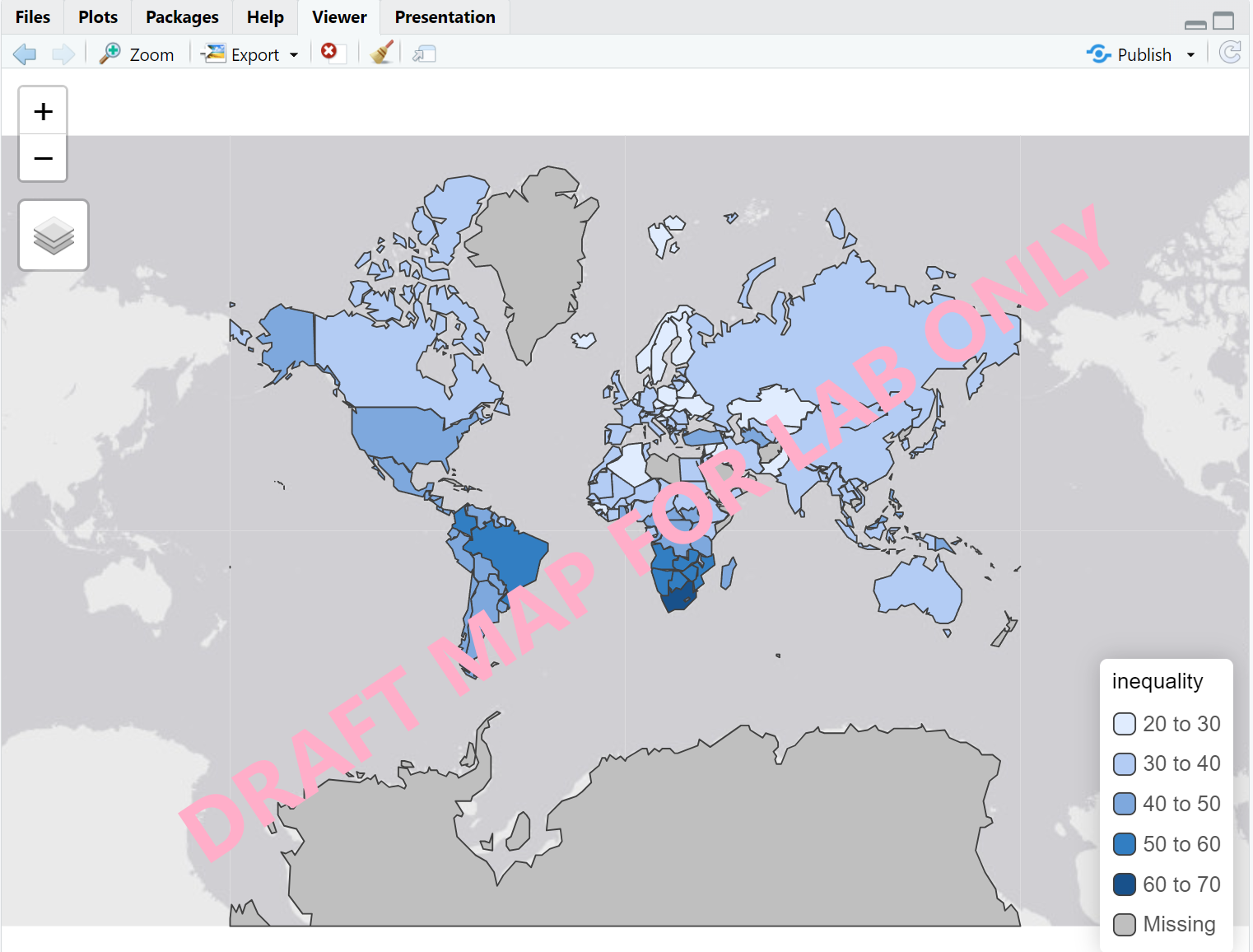
Next, we create a world map based on their level of inequality.
Please run the command below on your local machine. What do you see
under the Plot tab on bottom right? You should see a
map similar to the screenshot below.
[Q] Click “Zoom” and capture a screenshot of the map and paste it to your “Lab1 Report”. Close the “Plot Zoom” window and go back to the script.
# create a map
tm_shape(World) +
    tm_polygons("inequality")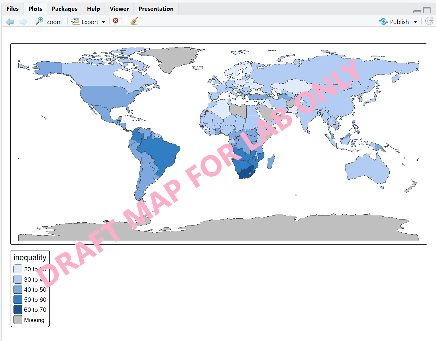
1.4.2 Interactive Map
Next, we will create an interactive map to explore countries’ happy planet index (HPI). The Happy Planet Index is a measure of sustainable well-being in considering human well-being and environmental impact.
We will use a different color palette (Yellow & Green) for this map. Type the code to your script –> select –> run.
tmap_mode("view")

tm_shape(World) +
    tm_polygons("HPI", palette = "YlGn")
[Q] Under the Plot tab, click
“Zoom”. Please do a screenshot of the map and paste it to your
“Lab1 Report”.
[Q] Hover over the map and click any country, you
should be able to see their HPI index. Please report HPI indexes of any
five countries to “Lab1 Report”.
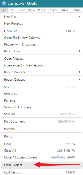
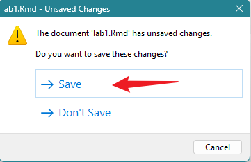
1.5. Close & Exit
To close an R project, please go “File”–> “Close Project” – a pop window asking “Do you want to save these changes” –> “Yes”.